Insurance Analysis

Synopsis

This dataset contains information from a collection of customers of a particular insurance agency. The customers currently have health insurance and I am interested in whether the variables in the current data set can be used to predict whether a customer is interested in expanding their insurance coverage to include their vehicle. The variable Response indicates whether a customer is interested in expanding their coverage (“Yes”) or not (“No”). After data processing and exploratory data analysis, I compared three models, a logistic regression, a penalized logistic regression and a random forest model. These models had similar performance and failed to correctly predict that a customer was interested in expanding their coverage. This is because the outcome variable, Response, is imbalanced. To address this I implemented 3 sampling techniques, upsampling, downsampling, and smote sampling, within a logistic regression. This offered significant improvements and a viable model. The most important factors in influencing a customers decision to expand their insurance covereage were whether they had been in a car accident recently, whether they already had car insurance, their age, and various selling strategies. This model offers insight into customer decision making and can help influence business decisions.

data<-read.csv("train.csv")
test<-read.csv("test.csv")

Data Preparation

Most of the variables are not of the proper type, so I will convert character variables to factors and recode some of them to have meaningful levels.

data<-data%>%
    mutate_if(is.character,as.factor)%>%
    mutate_at(c("Driving_License","Previously_Insured","Response","Region_Code",
                "Policy_Sales_Channel"),as.factor)

data$Response<-recode_factor(data$Response, `0` = "No",
                              `1` = "Yes")
data$Vehicle_Damage<-recode_factor(data$Vehicle_Damage,No="No Damage",
                                    Yes="Damage")
data$Previously_Insured<-recode_factor(data$Previously_Insured,`0`="No Insurance",
                                        `1`="Insurance")
data$Driving_License<-recode_factor(data$Driving_License,`0`="No DL",
                                     `1`="Has DL")

test<-test%>%
    mutate_if(is.character,as.factor)%>%
    mutate_at(c("Driving_License","Previously_Insured","Region_Code",
                "Policy_Sales_Channel"),as.factor)

test$Vehicle_Damage<-recode_factor(test$Vehicle_Damage,No="No Damage",
                                    Yes="Damage")
test$Previously_Insured<-recode_factor(test$Previously_Insured,`0`="No Insurance",
                                        `1`="Insurance")
test$Driving_License<-recode_factor(test$Driving_License,`0`="No DL",
                                     `1`="Has DL")

Create validation/training data sets

Since this particular set of data already has a separate csv file for the test data set, I will split the training dataset to create a validation set. So as to be able to test the models and avoid overfitting.

set.seed(1111)
split<-initial_split(data,prop=.7,strata=Response)
train<-training(split)
valid<-testing(split)

Exploratory Data Analysis

skim(train)

Data summary

Name	train
Number of rows	266775
Number of columns	12
_______________________
Column type frequency:
factor	8
numeric	4
________________________
Group variables	None

Variable type: factor

skim_variable	n_missing	complete_rate	ordered	n_unique	top_counts
Gender	0	1	FALSE	2	Mal: 144387, Fem: 122388
Driving_License	0	1	FALSE	2	Has: 266222, No : 553
Region_Code	0	1	FALSE	53	28: 74493, 8: 23602, 46: 13828, 41: 12783
Previously_Insured	0	1	FALSE	2	No : 144731, Ins: 122044
Vehicle_Age	0	1	FALSE	3	1-2: 140256, < 1: 115282, > 2: 11237
Vehicle_Damage	0	1	FALSE	2	Dam: 134854, No : 131921
Policy_Sales_Channel	0	1	FALSE	153	152: 94318, 26: 55864, 124: 51861, 160: 15132
Response	0	1	FALSE	2	No: 234079, Yes: 32696

Variable type: numeric

skim_variable	n_missing	complete_rate	mean	sd	p0	p25	p50	p75	p100	hist
id	0	1	190731.66	110028.23	4	95404	190759	286113.5	381107	▇▇▇▇▇
Age	0	1	38.82	15.50	20	25	36	49.0	85	▇▅▃▂▁
Annual_Premium	0	1	30553.58	17164.73	2630	24403	31671	39411.0	540165	▇▁▁▁▁
Vintage	0	1	154.23	83.64	10	82	154	227.0	299	▇▇▇▇▇

This summary shows a few things of interest. First is that there are no missing value. Second is that the outcome variable is quite unbalanced with the majority of individuals being not interested (~88%). This can have an effect on model performance, and various sampling techniques (e.g. upsample/smote) will be implemented. The Driving_license predictor is also very unbalanced with a tiny subset of individuals having no driver’s license, thus this predictor may not be very useful. There are also a relatively small proportion of individuals in this sample with a car age greater than 2 years. The other factor variables seem to have a relatively even balance of responses in their different levels. The numeric variables such as age seem to be within a reasonable range. Both Region_Code and Policy_Sales_Channel have many unique values so some of the less frequent categories may need to be consolidated in order to reduce dimensionality and uninformative categories.

EDA of Numeric Predictors

library(GGally)

train%>%
  select(Age,Annual_Premium,Vintage,Response)%>%
  ggpairs(mapping=aes(color=Response,alpha=.5),title="Numeric Predictors as a Function of Response")+
  theme(plot.title = element_text(hjust=.5))+
  scale_color_brewer(type="qual",palette="Dark2")+
  scale_fill_brewer(type="qual",palette="Dark2")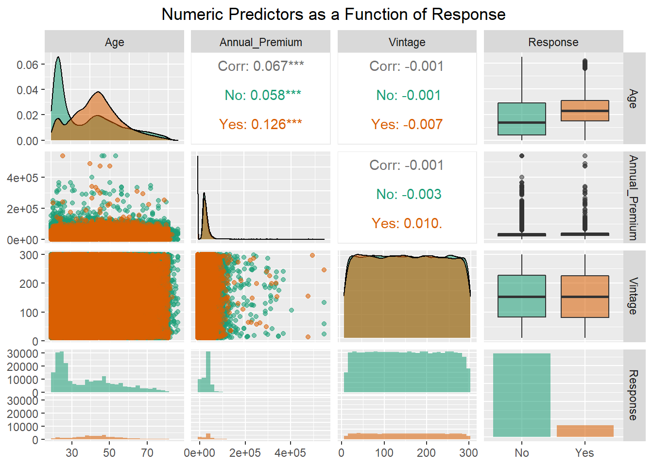

This plot shows that age has a skewed bimodal distribution for “No” respondents with the majority of individuals being around 25 years of age, and another concentration of individuals around 40 years of age. For “Yes” respondents, the distribution is less bimodal with the majority of responses centered around customers who are 40 years old. Examining the boxplot of Age shows that the median age of customers responding yes is older than those who responded no. The annual premium is also skewed with individuals who responded yes and no seemingly having a similar distribution of premiums. As was seen in the summary there is a maximum annual premium of 540,165, which is far above the median value of 31,662. The number of days with the company is an almost uniformly distributed predictor with no difference between “Yes” and “No” customers. The correlations among the predictors shows that there is little to no relationship among these numeric predictors indicating the absence of multicolinearity. This is important to keep in mind as the response variable is binary and thus logistic regression is a prime model of interest and one of the model assumptions is that there is no multicolinearity.

Categorical Bar Charts

Insurance Expansion as a function of vehicle age and current Insurance status

catp1<-ggplot(data=train,aes(x=Vehicle_Age,fill=Response))+
    geom_bar(position="dodge")+
    scale_fill_brewer(type="qual",palette="Dark2")+
    facet_wrap(~Previously_Insured)+
    labs(title="New Car Insurance as a Function of Current Insurance and Vehicle Age",
         x="Vehicle Age",
         fill="Purchase New \nInsurance?")+
    theme(plot.title = element_text(hjust=.5))
ggplotly(catp1,width=800)

This plot indicates that customers with vehicle insurance are not indicating that they want to purchase car insurance. This is seems quite intuitive and unsurprising so it is good that the data backs this notion up. Among those without car insurance, it seems that customers with cars between 1 and 2 years old purchase car insurance much more frequently than customers with cars that are less than 1 year or greater than 2 years old.

Insurance expansion as a function of gender and driver’s license possesion

catp2<-ggplot(data=train,aes(x=Gender,fill=Response))+
    geom_bar(position="dodge")+
    facet_wrap(~Driving_License)+
    scale_fill_brewer(type="qual",palette="Dark2")+
      labs(title="New Car Insurance as a Function of Gender and Driver's License (DL)",
         fill="Purchase New \nInsurance?")+
    theme(plot.title = element_text(hjust=.5))
ggplotly(catp2,width=800)

This plot first and foremost shows that there are not many customers without a Driver’s License. In addition to this there is not much difference among men and women in terms of responding yes and no. Both men and women respond yes and no in similar proportions. Thus possession of a driver’s license is not a very useful predictor since only one level has the majority of observations.

Boxplots of insurance expansion as a function of vehicle age and current insurance status

Since customer Age, Vehicle Age, and current car insurance seem to be useful predictors, I want to examine how all of these interact.

bp1<-ggplot(data=train,aes(x=Vehicle_Age,y=Age,fill=Response))+
    geom_boxplot(position=position_dodge(1))+
    facet_wrap(~Previously_Insured)+
    scale_fill_brewer(type='qual',palette="Dark2")+
        labs(title="New Car Insurance as a Function of Age, Current Insurance, and Vehicle Age ",
         x="Vehicle Age",
         fill="Purchase New \nInsurance?")

ggplotly(bp1,width=800)%>%
    layout(boxmode="group")

This plot indicates that the age distribution is quite similar among customers who respond yes or no to new car insurance purchases across both vehicle age and current car insurance status. The main difference in yes and no responses comes with customers who do not currently have car insurance and have a vehicle less than one year old. In this case, customers who respond yes seem to be older than those who respond no.

EDA Summary

Using these plots and summary techniques I was able to glean a few interesting things from the data.

1. There is a large class imbalance in the outcome variable (Response)
2. Age, Vehicle Age, and Current Car Insurance Status seem to be informative predictors
3. Multicolinearity among the predictors is not present
4. Some categorical predictors have either few responses in one category (Driver’s License) or have many categories that need to be consolidated (REgion code and Policy Sales Channel)

Machine Learning Models

For this data set I am going to be comparing 3 different models, logistic regression, penalized logistic regression, and random forest. All 3 models can handle this binary classification problem but have various pros and cons associated with them.

Logistic Regression

• Pros
  • Easy interpretation and implementation
  • Computationally efficient
  • Less inclined to overfit low dimensional data
• Cons
  • Has assumptions that must be met to have reliable parameter estimates
  • Tends to overfit high dimensional data
  • Performs best when there is a linear relationship between predictors and logit of outcome variable
  • Doesn’t naturally capture complex relationships among predictors (e.g. interactions must be specified)

Penalized Logistic Regression

• Pros
  • Same as logistic regression but can accomodate highly correlated predictors with penalty/mixture parameters
  • Avoids overfitting with high dimensional data
  • Acts as an automatic feature selection method
• Cons
  • Additional hyperparameters require extra model tuning
  • Results are not as easy to interpret
  • It can be difficult to understand why certain predictors are penalized

Random Forest

• Pros
  • Very powerful predictive capabilities due to ensemble of trees and random selection of predictors
  • Automatically calculates interactions between predictors
  • Can examine non-linear relationships between predictors and outcome variable
• Cons
  • Computationally intensive due to large number of trees being aggregated
  • Requires hyperparameter tuning that takes additional time
  • Lack of model interpretability

Data Preparation

To prepare the data for modelling I first update the role of the ID variable so that it is included in the dataset but is not used in the modelling. Then I use step other to clump together categories in factors that have few observations (less than 1% of the data). This will help reduce the dimensionality of the data and increase how informative factor levels with few observations are. Step novel prepares the data set so that if the test data set has new category levels not seen in the training data set, these additional levels with be stored under a “new” label. This simply helps models not experience any warnings or errors when they are applied to the test data set. I apply a logarithmic transformation of the annual premium predictor as it is heavily skewed, and I did not want to remove a substantial amount of outliers.
I normalize the data (subtract each value from the mean and divide by the SD) to make sure all predictors are on the same scale so large values don’t incorrectly bias parameter estimates. Then the logistic regression models require the factor predictors to be converted to dummy variables. Next I use step nsv to remove any predictors that are highly unbalanced such as the driver’s license predictor. Using the freq_cut argument I specify the ratio of the most frequent level to the second most frequent value. I specify this ratio to be 99 to 1 (i.e. out of 100 samples, 99 are for the first class and 1 is for the second class) so that a predictor with a ratio greater than this is removed. This is more conservative than the default value as I lean towards keeping data when I can help it. Finally, I create cross-validation folds which will be used to further reduce the likelihood of the models overfitting.

levels(train$Response)<-c("No","Yes")
insurance_recipe<-recipe(Response~.,data=train)%>%
    update_role(id,new_role = "ID")%>%
    step_other(all_nominal_predictors(),threshold=.01)%>%
    step_novel(all_nominal_predictors())%>%
    step_log(Annual_Premium)%>%
    step_normalize(all_numeric_predictors())%>%
    step_dummy(all_nominal_predictors())%>%
    step_nzv(all_predictors(),freq_cut = 99/1)

# create cross validation sets to reduce model variance
cv_folds<-vfold_cv(train,v=5)

Setting up model engines and hyperparameter tuning

Using tidymodels for my model specification I set the mode to classification for all models (although this is not necessary for logistic regression). For the penalized logistic regression, I use the glmnet engine which fits a logistic regression with a mixture of Lasso (L1) and Ridge (L2) regularization. Lasso regularization adds a an extra term to the logistic regression loss function that multiplies a penalty term (aka alpha) by the absolute value of the model coefficients. Ridge regularization on the other hand, adds an extra term that multiplies a penalty term by the squared value of the model coefficients. Ridge regularization is preferable when all coefficients should be incorporated into the model as it “pushes” less informative coefficient values close to zero. Lasso regularization forces these less informative coefficient values to be zero. Glmnet has the ability to combine the two of these regularization techniques to make an elastic net regularization. This results in some coefficients being shrunk towards zero (L2) and others being set to zero (L1). There are two hyperparameters that I am going to tune with the penalized model, penalty and mixture.

• The penalty parameter (alpha) affects how much coefficient values are minimized
• The mixture parameter (lambda) ranges from 0 to 1 with 0 being full Ridge regularization and 1 being full Lasso regularization

For the Random Forest model, I am using the ranger engine as it is an efficient implementation of the random forest model. There are two hyperparameters I am tuning for this model mtry and trees.

• mtry refers to the number of predictors that the random forest model will consider at each split.
• trees refers to how many trees are to be used

lr_mod<-logistic_reg()%>%
    set_mode("classification")%>%
    set_engine("glm")

lr_mod_RL<-logistic_reg(penalty=tune(),mixture=tune())%>%
    set_engine("glmnet")%>%
    set_mode("classification")

rf_mod<-rand_forest(mtry=tune(),trees=tune())%>%
    set_mode("classification")%>%
    set_engine("ranger")

Specifying hyperparameter tuning grid

For the hyperparameter tuning grid I am letting the tune function specify the range for the penalized logistic regression. This tidymodels function selects reasonable endpoints for each parameter. For example, the mixture parameter has a range from 0-1. With 7 levels (including endpoints) for each parameter there will be 49 models compared.

For the random forest model I specify the hyperparameter endpoints as these are values I am interested in testing. There are a total of 4 levels across the tuning grid for the random forest with all parameter combinations implemented resulting in 16 models.

lr_grid<-grid_regular(penalty(),
                      mixture(),
                      levels=7)
rf_grid<-grid_regular(mtry()%>%range_set(c(1, 10)),
                      trees()%>%range_set(c(500,2000)),
                      levels=4)

Making workflow to allow easy interchange of the models

insurance_wf<-workflow() %>%
    add_recipe(insurance_recipe,
               blueprint = hardhat::default_recipe_blueprint(allow_novel_levels = TRUE))%>%
    add_model(lr_mod)

Model Fitting

For the model fits I am collecting 3 different metrics F-score, Accuracy and the roc_auc score. To understand how these metrics are calculated, it is necessary to understand confusion matrices. Confusion matrices (like the one below) are a way of displaying the results of a classification problem to assess model performance.

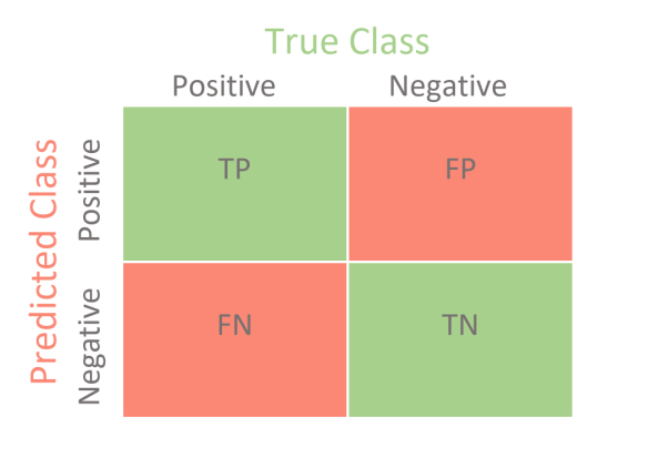
Example Confusion Matrix

In this example the model predictions are presented on the Y-axis and the actual data values are presented on the X-axis. The positive and negative values are arbitrary names that correspond to the outcome variable classes (e.g. “No” and “Yes”). There are 4 different classification outcomes:

• True Positive (TP): When the model correctly predicts an observation as Positive
• True Negative (TN): When the model correctly predicts an observation as Negative
• False Positive (FP): When the model incorrectly predicts an observation as Positive when it’s true value is Negative (aka type I error)
• False Negative(FN): When the model incorrectly predicts an observation as Negative when it’s true value is Positive (aka type II error)

With these values, various metrics can be calculated that can be used to evaluate different weakness in a model fit

• Recall (aka Sensitivity or True Positive Rate): This is an important metric when the reduction of false negative is key to the question of interest \[ \frac{TP}{TP+FN} \]

• Specificity: This metric is important when correctly categorizing the negative category is of the utmost importance
  \[ \frac{TN}{TN+FP}\]

• Precision: This metric is important when false positives are undesireable and we want to be confident in the positive predicted values \[\frac{TP}{TP+FP}\]

• Accuracy: The most common metric for classification model performance as it measures how well the model
  correctly classifies observations. Not a good metric when class imbalance is a concern. \[ \frac{TP+TN}{TP+FN+FP+TN}\]

• Receiver Operating Characteristic Curve/Area Under the Curve (ROC/AUC): The ROC curve plots the true positive rate against the false positive rate. The false positive rate is calculated as 1-Specificity.

  

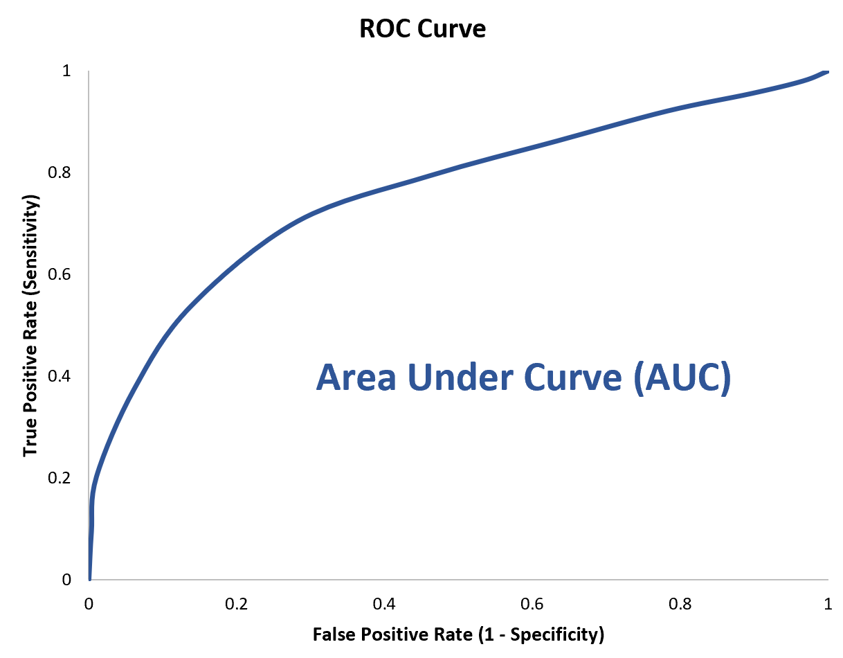
  Example ROC Curve

  This is a useful measure in classification problems as it can measure model biases at different thresholds. The AUC is a related metric that measures the area under this entire curve to provide an aggregate measure across all classification thresholds. This is the value returned by the roc_auc metric. This can range from 0-1 with 0 indicating the model predictions are all incorrect, and a value of 1 indicating the model has perfect classification.

• F-Score (f_meas): This metric is when we are interested in the trade off between precision and recall.\[\left(1+\beta^{2}\right)*\frac{Precision*Recall}{\beta^{2}*Precision+Recall}\] The \(\beta\) parameter can allow the user to specify the importance of recall over precision. For example, a value of 2 indicates that recall is twice as important as precision. If the \(\beta\) value is 1 then the F1-score is calculated which is the harmonic mean of precision and recall and is useful when a balance between these two metrics is required. This is of particular interest when false negatives are a concern. \[\frac{2*Precision*Recall}{Precision+Recall}\]

Logistic Regression Model Fit

lr_fit_train<- insurance_wf%>%
    fit_resamples(resamples=cv_folds,
                  metrics = metric_set(
                      f_meas,
                      accuracy,
                      roc_auc),
                  control = control_resamples(save_pred = TRUE))

Penalized Logistic Regression Model fit-hyperparameter tuning

insurance_wf<-update_model(insurance_wf,lr_mod_RL)
lr_pen_fit<-insurance_wf%>%
    tune_grid(resamples=cv_folds,
                  grid=lr_grid,
                      metrics = metric_set(
                      f_meas,
                      accuracy,
                      roc_auc),
                  control=control_grid(save_pred=TRUE))

Penalized Regression Hyperparameter fit visualization

lr_pen_fit %>%
  collect_metrics() %>%
  mutate(mixture = factor(mixture)) %>%
  filter(mean>.8)%>%
  ggplot(aes(penalty, mean, color = mixture)) +
  geom_line(size = 1.2, alpha = 0.5) +
  geom_point(size = 2) +
  facet_wrap(~ .metric, scales = "free_y", nrow = 2) +
  scale_x_log10(labels = scales::scientific,limits=c(NA,.05)) +
  scale_color_viridis_d(begin = .9, end = 0)+
  ggtitle("Penalized Logistic Regression Hyperparameters")+
  theme(plot.title = element_text(hjust=.5))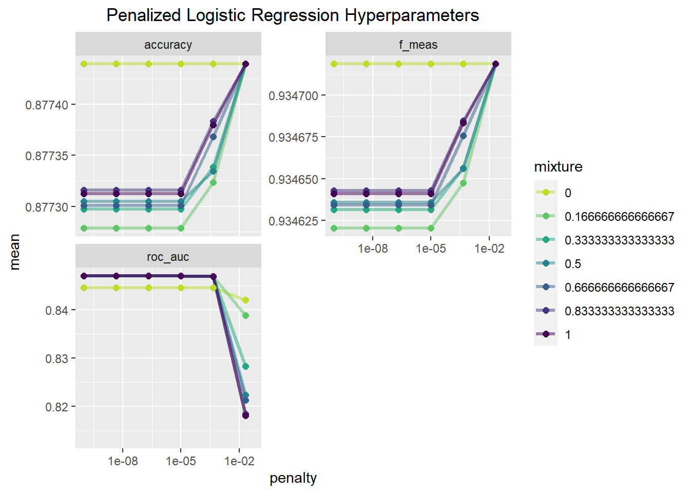

This set of plots indicates that a mixture value of zero seems to provide the best fitting model across all penalty values for accuracy and the F-measure. Mixture values other than zero achieve a similar level of accuracy and F-score when the penalty is large. In relation to the AUC value, the model with a mixture a value of 0 does worse until the penalty value is relatively large, and then it is the best. That being said the difference in performance between these hyperparameter values is very small, differing by values in the ten thousandths for the most part. Since AUC is the main metric of interest, I will put more weight on that in making my modelling choice.

lr_pen_best<-select_best(lr_pen_fit,metric = "roc_auc")
show_best(lr_pen_fit,metric="roc_auc")

## # A tibble: 5 x 8
##         penalty mixture .metric .estimator  mean     n  std_err .config         
##           <dbl>   <dbl> <chr>   <chr>      <dbl> <int>    <dbl> <chr>           
## 1 0.0000000001    0.167 roc_auc binary     0.847     5 0.000861 Preprocessor1_M~
## 2 0.00000000464   0.167 roc_auc binary     0.847     5 0.000861 Preprocessor1_M~
## 3 0.000000215     0.167 roc_auc binary     0.847     5 0.000861 Preprocessor1_M~
## 4 0.00001         0.167 roc_auc binary     0.847     5 0.000861 Preprocessor1_M~
## 5 0.0000000001    0.333 roc_auc binary     0.847     5 0.000868 Preprocessor1_M~

This function shows that the best model based on AUC is one with a mixture of 1/6 and a penalty of 1e^-10 which will be the penalized logistic regression model I use going forward.

Random Forest Model Fit

Although the random forest model does not require dummy variables I will still use the same recipe as the logistic regression for the sake of simplicity.

set.seed(1234)
insurance_wf<-update_model(insurance_wf,rf_mod)
RF_fit<-insurance_wf%>%
    tune_grid(resamples=cv_folds,
                  grid=rf_grid,
                  metrics = metric_set(
                      f_meas,
                      accuracy,
                      roc_auc),
                  control=control_grid(save_pred = TRUE)
              )

Random Forest Hyperparameter fit visualization

RF_fit %>%
  collect_metrics() %>%
  mutate(mtry = factor(mtry)) %>%
  ggplot(aes(trees, mean, color = mtry)) +
  geom_line(size = 1.2, alpha = 0.5) +
  geom_point(size = 2) +
  facet_wrap(~ .metric, scales = "free", nrow = 2) +
  scale_color_viridis_d(begin=.9,end=0)+
  ggtitle("Random Forest Hyperparameters")+
  theme(plot.title = element_text(hjust=.5))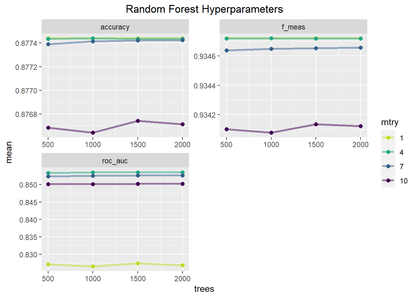

This plot shows how performance metrics change as a function of the number of trees and the number of randomly sampled predictors at each split. Across all metrics an mtry value of 7 or 10 performs the worst and is relatively unaffected by the number of trees. mtry of 1 and 4 are nearly equivalent for accuracy and the f1-score with the mtry of 1 possibly being slightly better. With AUC, mtry of 4 consistently outperforms the other mtry possibilities. The number of trees seems to have little influence on the model performance, with a slight increase from 500-1000 trees but above that seems to offer no benefit. The table below will show the best parameter combinations based on AUC.

rf_best_fit<-select_best(RF_fit,metric="roc_auc")
show_best(RF_fit,metric="roc_auc")

## # A tibble: 5 x 8
##    mtry trees .metric .estimator  mean     n  std_err .config              
##   <int> <int> <chr>   <chr>      <dbl> <int>    <dbl> <chr>                
## 1     4  1500 roc_auc binary     0.854     5 0.000847 Preprocessor1_Model10
## 2     4  2000 roc_auc binary     0.854     5 0.000862 Preprocessor1_Model14
## 3     4  1000 roc_auc binary     0.854     5 0.000844 Preprocessor1_Model06
## 4     4   500 roc_auc binary     0.853     5 0.000817 Preprocessor1_Model02
## 5     7  2000 roc_auc binary     0.853     5 0.000990 Preprocessor1_Model15

Model comparison

For the model comparison, I examine the confusion matrices and the ROC curve.

lr_pred<-
    lr_fit_train%>%
    collect_predictions()

lr_pen_pred<-
    lr_fit_train%>%
    collect_predictions(parameters=lr_pen_best)

rf_pred<-
    RF_fit%>%
    collect_predictions(parameters=rf_best_fit)

Confusion Matrices

cm_lr<-lr_pred%>%
    conf_mat(Response,.pred_class)%>%
    autoplot(type='heatmap')+
    ggtitle("Logistic Regression")
cm_lr_pen<-lr_pen_pred%>%
    conf_mat(Response,.pred_class)%>%
    autoplot(type='heatmap')+
    ggtitle("Penalized Regression")
cm_rf<-rf_pred%>%
    conf_mat(Response,.pred_class)%>%
    autoplot(type='heatmap')+
    ggtitle("Random Forest")
    
grid.arrange(cm_lr,cm_lr_pen,cm_rf,ncol=3,heights=c(1,1))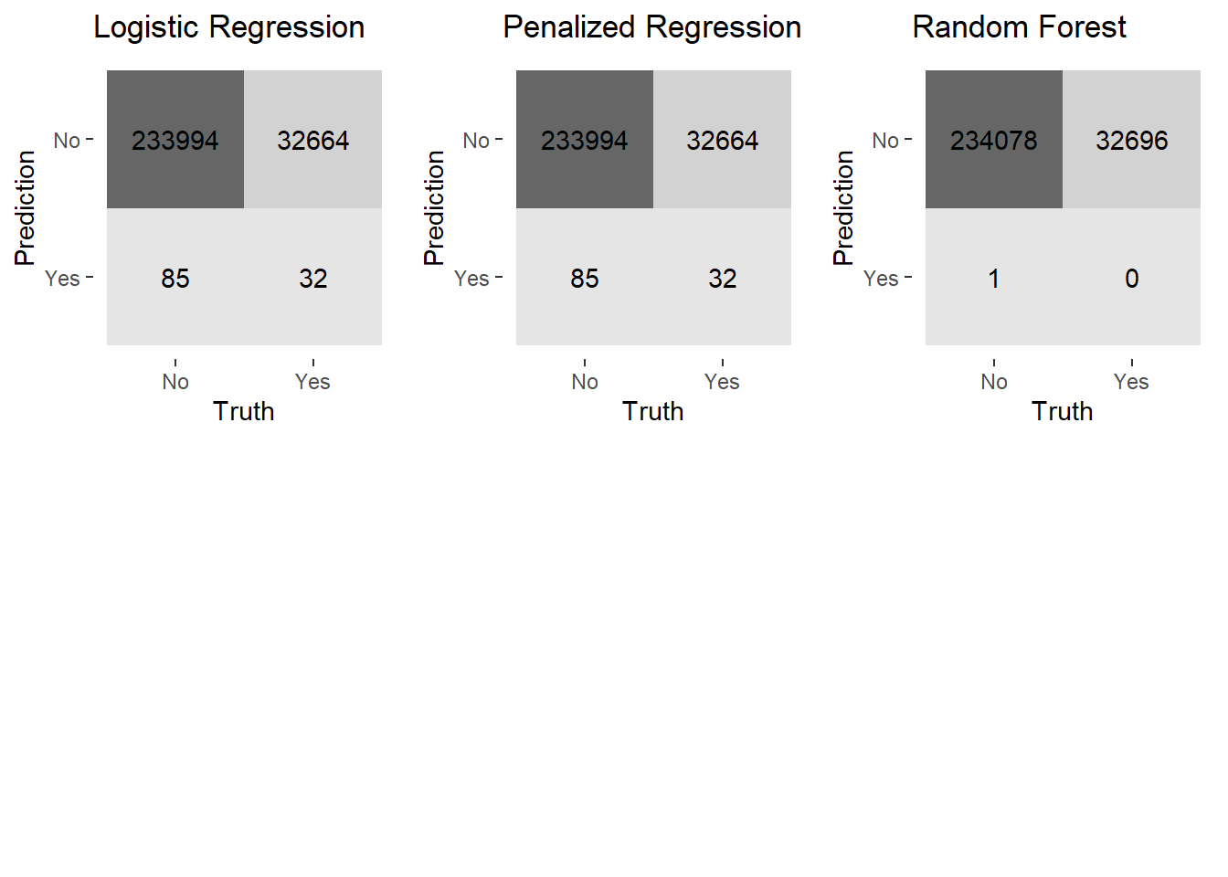

This plot of confusion matrices demonstrates a huge problem across all the models. The models are quite good at capturing true positives (a predicted “No” response in agreement with the actual data) but fails to capture the true negatives (a predicted “Yes” response in agreement with the actual data). All the models make an abundance of false positives (a predicted “No” response when the data is a “Yes” response) which is quite problematic since I am interested in developing a model that can capture the “Yes” responses. This is due to the unbalanced nature of the outcome variable. Even with a more powerful model technique such as random forest, there is still this issue present. To address this I will implement upsampling, downsampling and smote sampling to find a method to address this. I will examine the specificity and ROC values of the already fit models to determine which model I will test these different sampling methods with first.

lr_spec<-
    lr_pred%>%
    spec(Response,.pred_class)%>%
    mutate(Model="Logistic Regression")
lr_pen_spec<-
    lr_pen_pred%>%
    spec(Response,.pred_class)%>%
    mutate(Model="Penalized Logistic Regression")
rf_spec<-
    rf_pred %>%
    spec(Response,.pred_class)%>%
    mutate(Model="Random Forest")

lr_auc<-
    lr_pred%>%
    roc_auc(Response,.pred_No)%>%
    mutate(Model="Logistic Regression")
lr_pen_auc<-
    lr_pen_pred%>%
    roc_auc(Response,.pred_No)%>%
    mutate(Model="Penalized Regression")
rf_auc<-
    rf_pred%>%
    roc_auc(Response,.pred_No)%>%
    mutate(Model="Random Forest")

Compare Specificity and ROC

spec_plot<-bind_rows(lr_spec,lr_pen_spec,rf_spec) %>% 
  ggplot(aes(x=.estimate,y = Model, color = as.factor(Model))) + 
  geom_point(size=3)+
  scale_color_brewer(type="qual",palette="Dark2")+
  labs(title="Specificity Across Models",x="Specificity",color="Model")+
  theme(plot.title = element_text(hjust=.5))

auc_plot<-bind_rows(lr_auc,lr_pen_auc,rf_auc) %>% 
  ggplot(aes(x=.estimate,y = Model, color = as.factor(Model))) + 
  geom_point(size=3)+
  scale_color_brewer(type="qual",palette="Dark2")+
  labs(title="AUC Across Models",x="AUC",color="Model")+
  theme(plot.title = element_text(hjust=.5))


grid.arrange(spec_plot,auc_plot,nrow=2)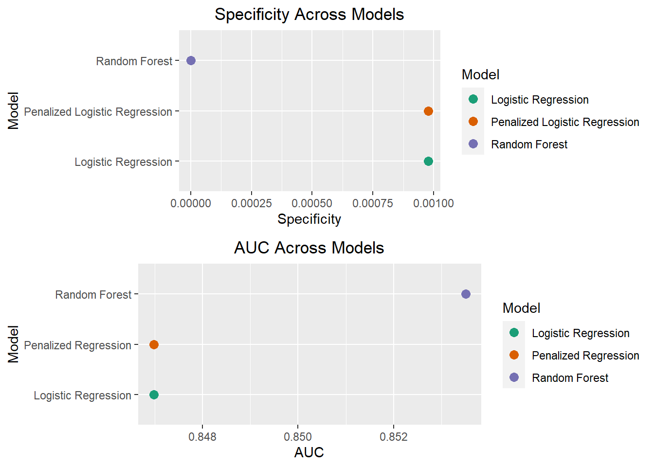

These plots show that the random forest model has both a slightly better AUC, but slightly worse specificity than the other models. Given there is not much of a performance improvement with the random forest model, I will be proceeding in my analyses with the base logistic regression model to test whether upsampling, downsampling or smote sampling will best address the class imbalance. Logistic regression also has the added benefit of being more interpretable, which will make it easier to implement business decisions based on the model.

Class Imbalance Modelling

To address the class imbalance I will be using 3 sampling techniques. I will briefly describe how each of these methods works.

1. Upsampling: This is a sampling technique in which cases from the minority class are sampled with replacement and added to the data set to create a more balanced ratio of the outcome variable classes.
   • In step_upsample, the parameter over_ratio controls the ratio of majority to minority class frequencies. A ratio of 1 indicates the minority class has the same number of observations as the majority class. A ratio of 2 would indicate the minority has twice as many observations as the majority class
2. Downsampling: This is a sampling technique in which cases from the majority class are removed at random to create a balanced ratio of the outcome variable classes.
   • In step_downsample, the parameter under_ratio controls the ratio of majority to minority class frequencies. A ratio of 1 indicates majority class observations are removed until it has the same frequency as the minority class. A ratio of 2 indicates the majority class observations are removed until they have at most twice the number of observations as the minority class.
3. Synthetic Minority Oversampling Technique (SMOTE): This is a type of upsampling in which novel observations are generated from the minority class using k nearest neighbors. The overall SMOTE algorithm works as follows:
   1. For each observation in the minority class, the k nearest neighbors will be calculated using a distance metric (e.g. Euclidean distance)
   2. A subset of these k nearest neighbors are sampled based on the over_ratio
   3. The distance between the observation and the selected nearest neighbor is calculated
   4. This distance is multiplied by a random number between 0 and 1
   5. The result of this multiplication is then added to the original observation to create a new observation The step_smote has two parameters over_ratio and neighbors. Neighbors refers to the number of neighbors in the k nearest neighbors part of the algorithm and over_ratio is the same previously described.

The main disadvantage of downsampling is that possibly important data is being thrown away, while with upsampling overfitting becomes more likely. SMOTE is a way to deal with the overfitting issue as the synthetic values are not the exact same values.

Add in sampling steps to recipes

library(themis)

upsamp_rec<-insurance_recipe%>%
  step_upsample(Response,over_ratio = tune())

downsamp_rec<-insurance_recipe%>%
  step_downsample(Response,under_ratio = tune())

smote_rec<-insurance_recipe%>%
  step_smote(Response,over_ratio=tune(),neighbors = tune())

Creating sampling tuning grids

I am doing a parameter search among a reasonable set of ranges at increments of 0.1.

upsamp_grid<-grid_regular(over_ratio()%>%range_set(c(.5,1.5)),
                          levels=11)
downsamp_grid<-grid_regular(under_ratio()%>%range_set(c(.5,1.5)),
                            levels=11)
smote_grid<-grid_regular(over_ratio()%>%range_set(c(.5,1.5)),
                         neighbors()%>%range_set(c(2,12)),
                         levels=11)

Upsample model

insurance_wf<-insurance_wf%>%
  update_recipe(upsamp_rec)%>%
  update_model(lr_mod)
set.seed(1111)
c1 <- makePSOCKcluster(5)
registerDoParallel(c1)

upsamp_lr_fit<-insurance_wf%>%
    tune_grid(resamples=cv_folds,
                  grid=upsamp_grid,
                      metrics = metric_set(
                      roc_auc,
                      spec,
                      sens,
                      f_meas),
                  control=control_grid(save_pred=TRUE,parallel_over = "resamples"))
stopCluster(c1)

Downsample model fit

set.seed(1234)
c1 <- makePSOCKcluster(5)
registerDoParallel(c1)

insurance_wf<-insurance_wf%>%update_recipe(downsamp_rec)
downsamp_lr_fit<-insurance_wf%>%
    tune_grid(resamples=cv_folds,
                  grid=downsamp_grid,
                      metrics = metric_set(
                      roc_auc,
                      spec,
                      sens,
                      f_meas),
                  control=control_grid(save_pred=TRUE,parallel_over = "resamples"))
stopCluster(c1)

Smote model fit

set.seed(9876)
c1 <- makePSOCKcluster(2)
registerDoParallel(c1)
insurance_wf<-insurance_wf%>%update_recipe(smote_rec)
smote_lr_fit<-insurance_wf%>%
    tune_grid(resamples=cv_folds,
                  grid=smote_grid,
                      metrics = metric_set(
                      roc_auc,
                      spec,
                      sens,
                      f_meas),
                  control=control_grid(save_pred=TRUE,parallel_over = "resamples"))
stopCluster(c1)

Model Evaluation

Upsample Model

These plots are the same as those presented earlier for the previous model fits.

upsamp_lr_fit %>%
  collect_metrics() %>%
  ggplot(aes(over_ratio, mean,color=mean)) +
  geom_point(size=2) +
  geom_line()+
  facet_wrap(~ .metric, scales = "free", nrow = 2) +
  scale_color_viridis_c(begin =.9,end=.1)+
  labs(x="Over Ratio Parameter Values",
       title = "Upsample Logistic Regression")+
  theme(plot.title=element_text(hjust=.5))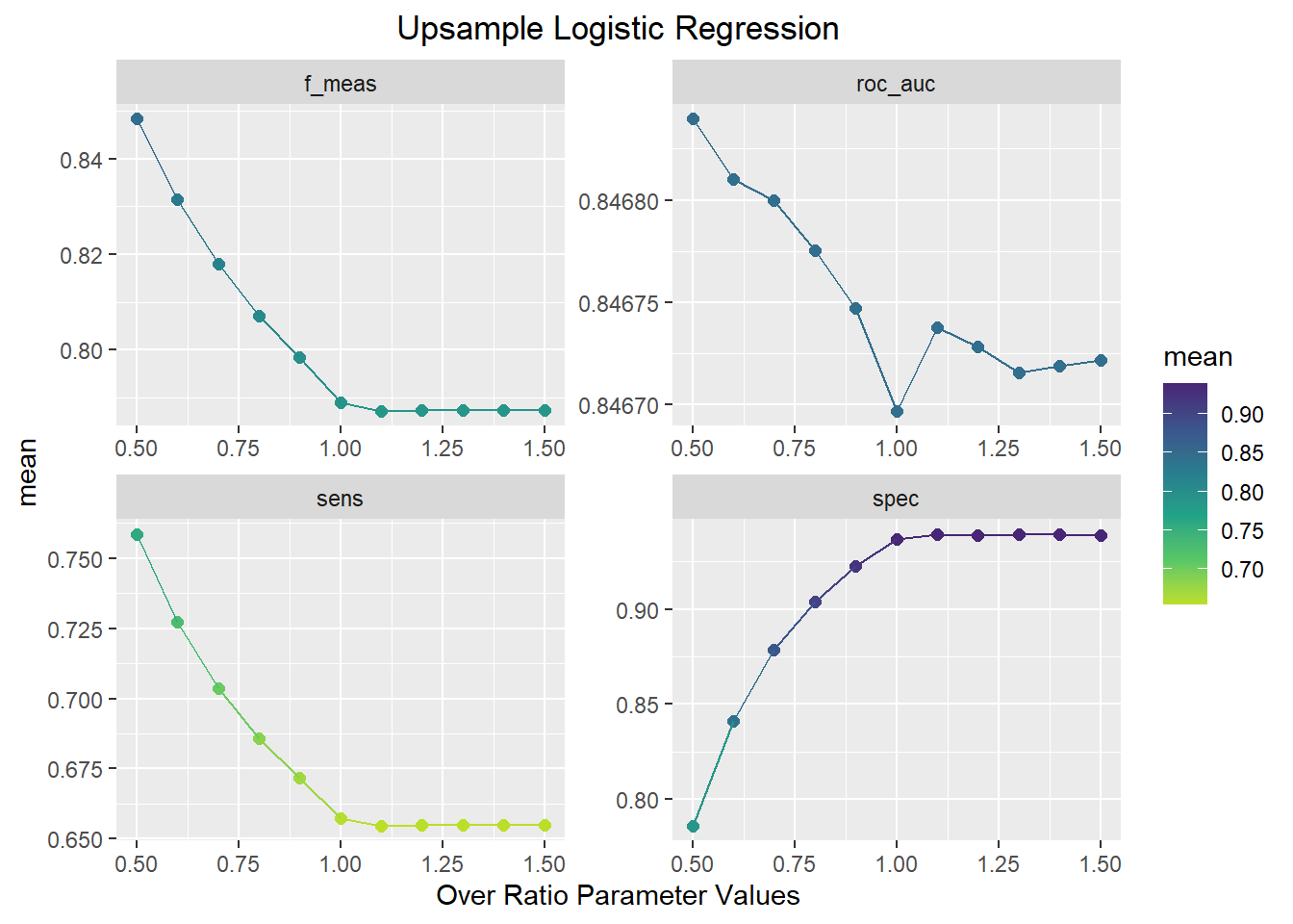

This plot shows that the best ROC and F1-score performance occurs when the over_ratio parameter is equal to 0.5. As the Over_ratio increases to 1.0, sensitivity, AUC, and F1-score decrease while specificity increases. With the over_ratio at 0.5, sensitivity and specificity are balanced and is a significant improvement over the previous methods.

Downsample Model

downsamp_lr_fit %>%
  collect_metrics() %>%
  ggplot(aes(under_ratio, mean, color=mean)) +
  geom_point(size=2) +
  geom_line()+
  facet_wrap(~ .metric, scales = "free", nrow = 2) +
  scale_color_viridis_c(begin =.9,end=.1)+
  labs(x="Under Ratio Parameter Values",
       title = "Downsample Logistic Regression")+
  theme(plot.title=element_text(hjust=.5))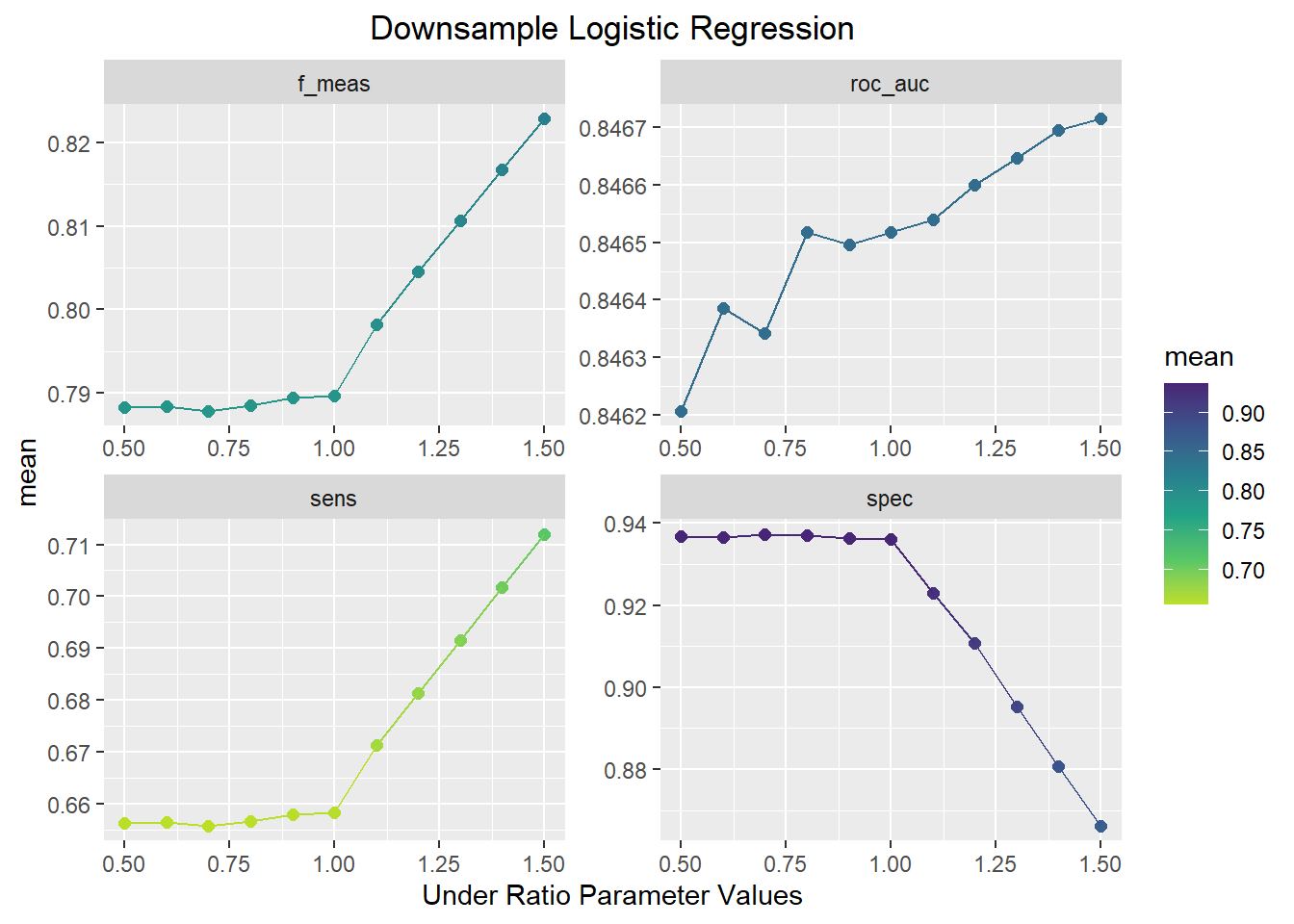

This plot shows the opposite pattern as the upsample model. In this plot, F1-score, AUC, and sensitivity increase and the specificity decreases as the under_ratio parameter increases. An under_ratio value of 1.5 seems to offer the best model performance.

Smote Model

smote_lr_fit %>%
  collect_metrics() %>%
  mutate(neighbors = factor(neighbors)) %>%
  ggplot(aes(over_ratio, mean, color=neighbors)) +
  geom_line(alpha=.5) +
  geom_point(size=2,alpha=.5)+
  facet_wrap(~ .metric, scales = "free", nrow = 2) +
  labs(x="Over Ratio Parameter Values",
       title = "Smote Logistic Regression",
       color="Neighbors Parameter \nValues")+
  theme(plot.title=element_text(hjust=.5))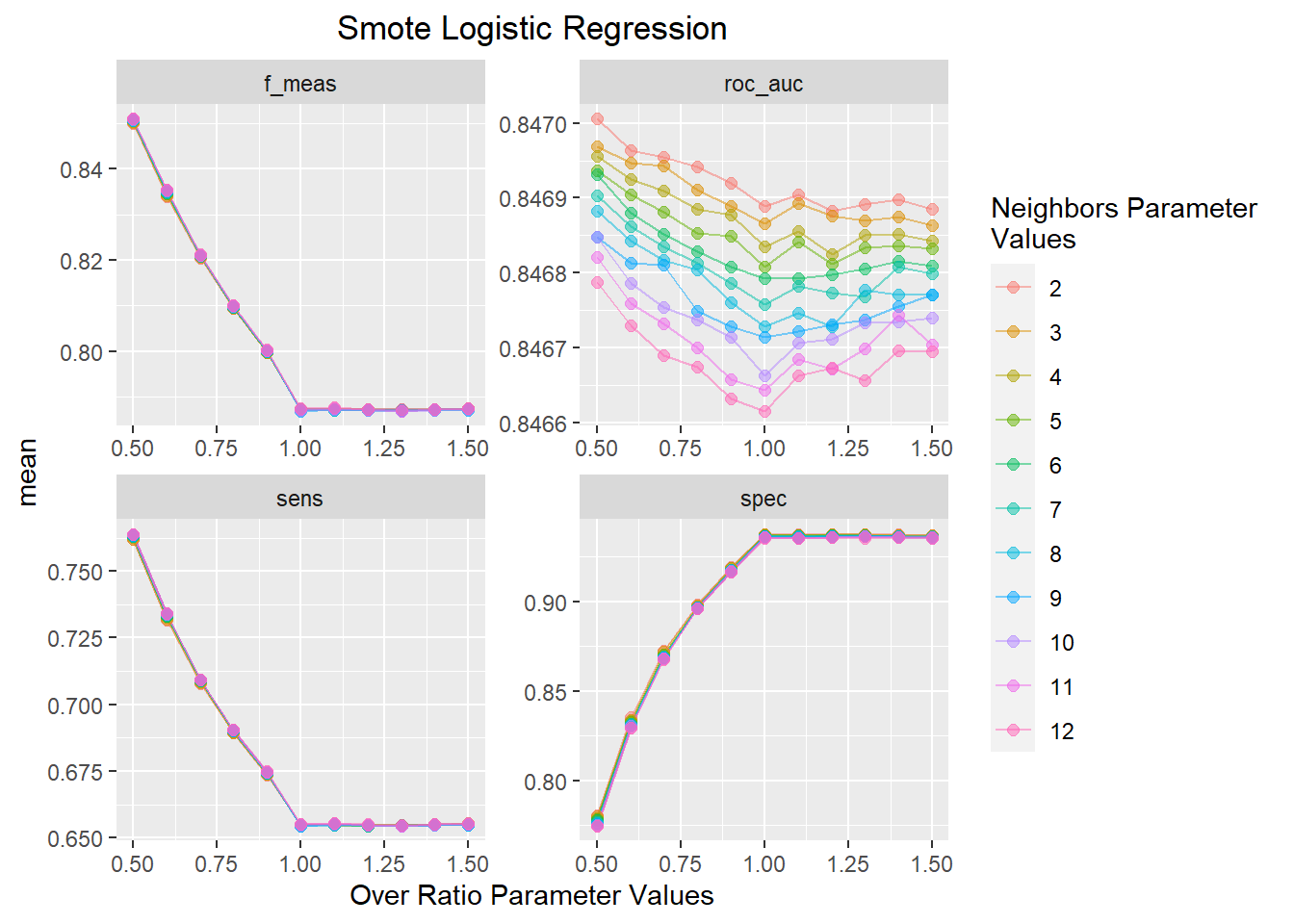

This plot shows a similar trend as the upsample model with sensitivity, AUC, and F1-score decreasing and specificity increasing as a function of increasing over_ratio values. The value of neighbors has a minimal effect on model performance with 2 neighbors offering the best AUC value across all over_ratio parameter values.

upsamp_best<-select_best(upsamp_lr_fit,metric='roc_auc')
downsamp_best<-select_best(downsamp_lr_fit,metric='roc_auc')
smote_best<-select_best(smote_lr_fit,metric='roc_auc')

upsamp_pred<-
    upsamp_lr_fit%>%
    collect_predictions(parameters=upsamp_best)

downsamp_pred<-
    downsamp_lr_fit%>%
    collect_predictions(parameters=downsamp_best)

smote_pred<-
    smote_lr_fit%>%
    collect_predictions(parameters=smote_best)

Confusion Matrices for sampling methods models

Using the parameters from the best fitting models I can now evaluate the model fit using a confusion matrix

cm_upsamp<-upsamp_pred%>%
    conf_mat(Response,.pred_class)%>%
    autoplot(type='heatmap')+
    ggtitle("Best Upsample")
cm_downsamp<-downsamp_pred%>%
    conf_mat(Response,.pred_class)%>%
    autoplot(type='heatmap')+
    ggtitle("Best Downsample")
cm_smote<-smote_pred%>%
    conf_mat(Response,.pred_class)%>%
    autoplot(type='heatmap')+
    ggtitle("Best Smote")
    
grid.arrange(cm_upsamp,cm_downsamp,cm_smote,ncol=3,heights=c(1,1))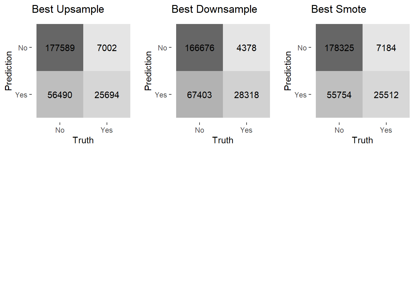

These confusion matrices show that all the sampling techniques result in fewer false negatives and many more false positives than with the previous models without sampling techniques implemented. These sampling models do make a lot of correct predictions that a customer will purchase more insurance, which is the result I was aiming for. Considering this is what I want the model to accomplish, this seems to be a vast improvement over the previous methods. The upsample model and smote model have similar performance, while the downsample model has more true negatives and false positives.

Test models with Validation set

Now that I have determined the sample techniques offer an improved fit, I will apply the best fitting models to the validation set to assess the model performance on data they were not trained on. This is the true test as a model needs to be able to perform well on unobserved data in order to be useful in practice.

upsamp_val_fit<-insurance_wf%>%
  update_recipe(upsamp_rec)%>%
  finalize_workflow(upsamp_best)%>%
  last_fit(split,metrics=metric_set(roc_auc,
           spec,
           sens))

downsamp_val_fit<-insurance_wf%>%
  update_recipe(downsamp_rec)%>%
  finalize_workflow(downsamp_best)%>%
  last_fit(split,metrics=metric_set(roc_auc,
           spec,
           sens))

smote_val_fit<-insurance_wf%>%
  update_recipe(smote_rec)%>%
  finalize_workflow(smote_best)%>%
  last_fit(split,metrics=metric_set(roc_auc,
           spec,
           sens))

ROC curves

up_curve<-upsamp_val_fit%>%
  collect_predictions()%>%
  roc_curve(Response,.pred_No)%>%
  mutate(Model="Best Upsample Model")

down_curve<-downsamp_val_fit%>%
  collect_predictions()%>%
  roc_curve(Response,.pred_No)%>%
  mutate(Model="Best Downsample Model")

smote_curve<-smote_val_fit%>%
  collect_predictions()%>%
  roc_curve(Response,.pred_No)%>%
  mutate(Model="Best Smote Model")

  bind_rows(up_curve,down_curve,smote_curve)%>%
  ggplot(aes(x = 1 - specificity, y = sensitivity, col = Model, lty=Model)) + 
  geom_path(lwd = 1, alpha = 0.8) +
  geom_abline(lty = 3) + 
  coord_equal() + 
  scale_color_viridis_d(option = "plasma", end = .8)+
  labs(title="ROC Curve All Sampling Models",
       x="False Positive Rate (1-Specificity)",
       y="True Positive Rate (Sensitivity)")+
  theme(plot.title = element_text(hjust=.5))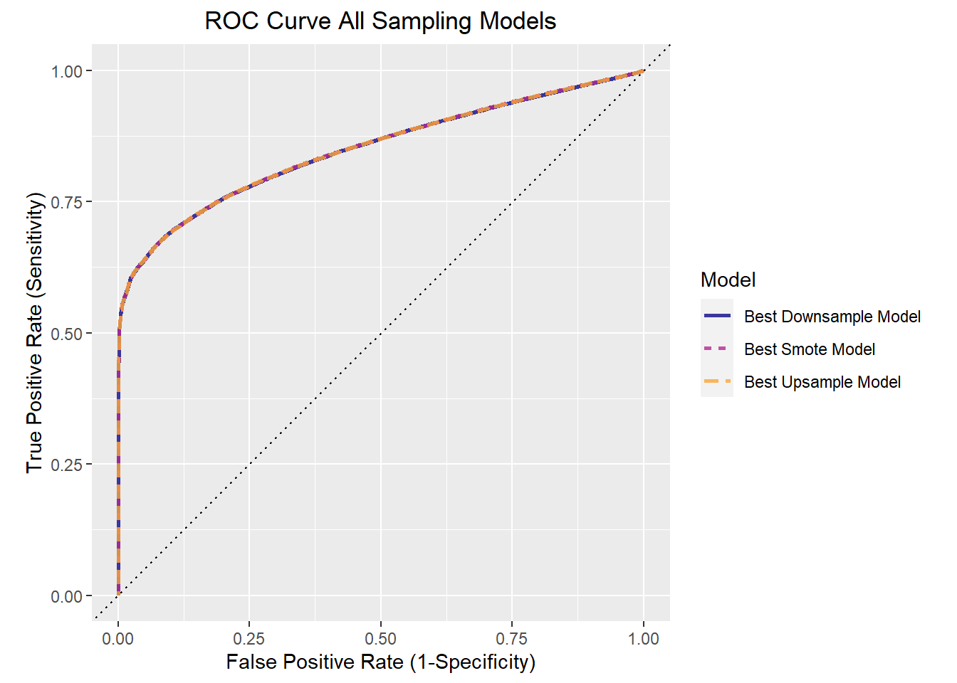

This ROC curve displays the tradeoff of the true positive rate (sensitivity) to the false positive rate (1-specificity). The three sampling techniques offer incredibly similar performance as can be seen with the lines overlapping.

Confusion matrices based on best decision cutoff

Since logistic regression provides the probabilities that an observation belongs to one class or another, the threshold at which an observation is classified into one class or another (e.g. No vs. Yes) has much influence on the model performance. The default value is .5, but this does not lead to the optimal tradeoff between the true positive rate and the false positive rate as can be seen in the ROC curve above. Different thresholds can be chosen depending on whether the true positive rate or false positive rate is of more interest. For my purposes I am looking for an equal balance between the two and thus I will be determining which threshold maximizes the true positive rate and the false positive rate. Different methods can be done to achieve this, but the one I have implemented is the simplest and most straightforward.

# This finds the most balanced decision threshold by maximizing the true positive rate 
#(sensitivity) minus the false positive rate (1-specificity)
up_curve_cut<- up_curve$.threshold[which.max(up_curve$sensitivity-(1-up_curve$specificity))]
down_curve_cut<- down_curve$.threshold[which.max(down_curve$sensitivity-(1-down_curve$specificity))]
smote_curve_cut<- smote_curve$.threshold[which.max(smote_curve$sensitivity-(1-smote_curve$specificity))]


cm_upsamp<-upsamp_pred%>%
    mutate(predclass=ifelse(upsamp_pred$.pred_No>up_curve_cut,"No","Yes"))%>%
    mutate(predclass=factor(predclass))%>%
    conf_mat(Response,predclass)%>%
    autoplot(type='heatmap')+
    ggtitle("Best Upsample")
cm_downsamp<-downsamp_pred%>%
    mutate(predclass=ifelse(downsamp_pred$.pred_No>down_curve_cut,"No","Yes"))%>%
    mutate(predclass=factor(predclass))%>%
    conf_mat(Response,predclass)%>%
    autoplot(type='heatmap')+
    ggtitle("Best Downsample")
cm_smote<-smote_pred%>%
    mutate(predclass=ifelse(smote_pred$.pred_No>smote_curve_cut,"No","Yes"))%>%
    mutate(predclass=factor(predclass))%>%
    conf_mat(Response,predclass)%>%
    autoplot(type='heatmap')+
    ggtitle("Best Smote")
    
grid.arrange(cm_upsamp,cm_downsamp,cm_smote,ncol=3,heights=c(1,1))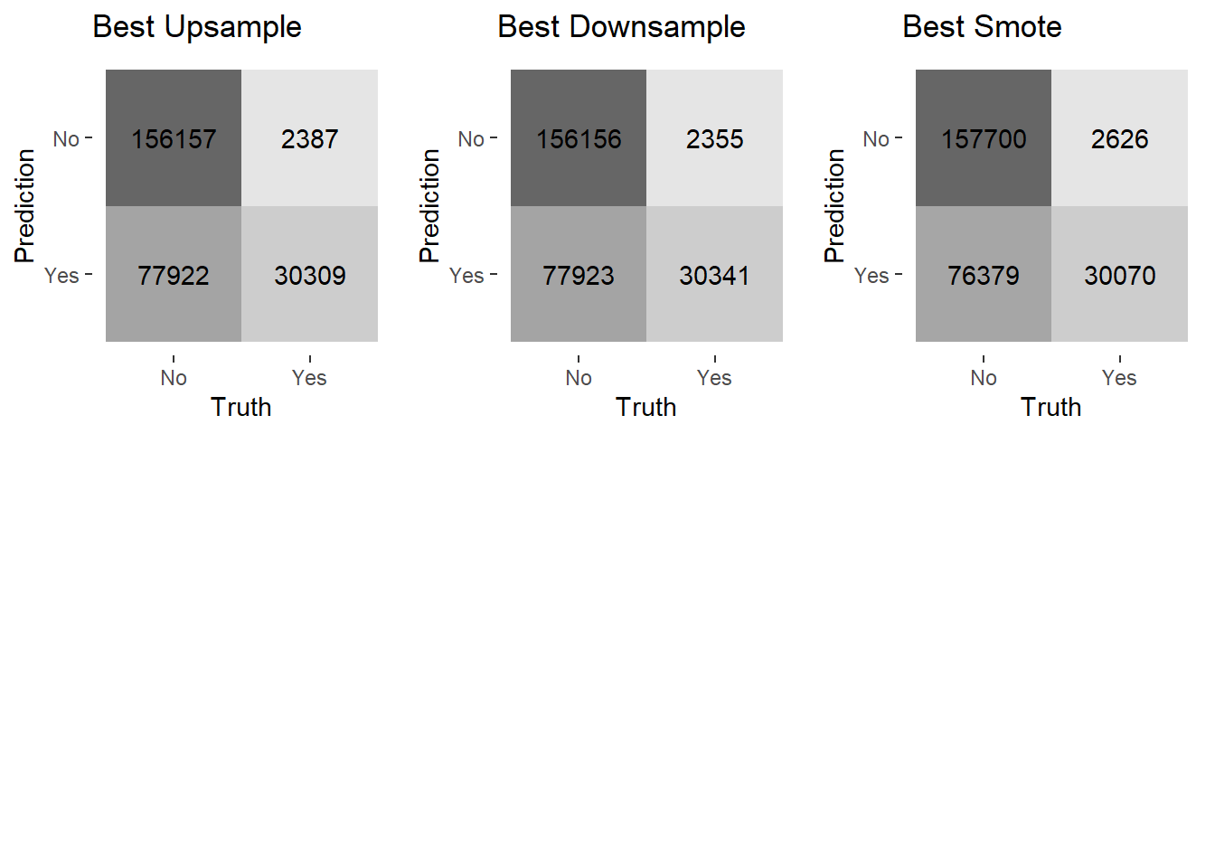

The optimal threshold for every model results in very similar performance. This is not surprising considering the ROC curves were overlapping. In relation to the previous confusion matrix on the training data, the models have a better rate of true negatives, more false positives, and fewer false negatives. This clearly is not the best model, but it offers a significant improvement over the initial efforts and can serve as a starting point in modelling efforts.

Final Model Fit

For the final fit, I am using the downsample model since the data set is very large and it offers similar performance to the other sampling techniques. Using this I will interpret the model coefficients to guide further decisions on how to divert resources to increase the amount of customers that expand their insurance coverage. Coefficients in logistic regression are given in terms of the log odds. However by exponentiating the coefficients I can convert this to the odds which is much easier to interpret.

downsamp_final<-insurance_wf%>%
  update_recipe(downsamp_rec)%>%
  finalize_workflow(downsamp_best)%>%
  fit(train)

Downsample Best Fitting Model Parameters

 downsamp_parm_plot<-extract_fit_parsnip(downsamp_final)%>%
   tidy(conf.int=TRUE,exponentiate=TRUE)%>%
   filter(p.value<.05&!term=="(Intercept)")%>%
   arrange(estimate)%>%
   ggplot(aes(x=estimate,y=term,color=term))+
   geom_point()+
   geom_vline(xintercept=1)+
   geom_errorbarh(aes(xmin=conf.low,xmax=conf.high))+
   labs(x="Estimate (Odds Ratio)",y="Model Parameter",title="Parameter Estimates with 95% Confidence Interval")+
   theme(legend.position="none")

 ggplotly(downsamp_parm_plot)

This plot shows the model coefficient estimates for the best fitting downsample logistic regression model. Only coefficients with a p-value less than .05 are included. The vertical black line indicates an odds ratio of 1 meaning the predictor is not informative. Unfortunately the actual values of the Region code and policy sales channel parameters were kept anonymous so I am unable to determine the specific sales method or region in which customers reside. The reference level for the policy sales channel is 26 while the reference level for region code is 2.

One of the strongest predictors is whether or not a customer has damaged their vehicle in the past. According to this model, the odds of a customer who has damaged their vehicle in the past to purchase new car insurance is 7 times higher than a customer who has not damaged their vehicle in the past. On the other end of the spectrum,if a customer already has vehicle insurance, they are incredibly unlikely to be interested in purchasing car insurance compared to customer without vehicle insurance. The way in which a customer is contacted for car insurance also plays a large role in whether they are interested in purchasing new car insurance or not. In particular, sales channels 160, 152, and 151 result in a customer being much less likely to purchase car insurance compared to sales channel 26. Thus, these sales techniques are having a detrimental impact and need to be abandoned or changed in some way. For age there is a negative relationship in which the odds of purchasing new car insurance decreases as customers age. Thus focusing marketing efforts on younger customers is a better use of resources. Most regions included in the predictor set increase the likelihood of purchasing new car insurance when compared to region 2. In particular, the odds of a customer in region 18 being interested in purchasing new car insurance is 2.5 times higher than a customer in region 2. Vehicle age also has an impact on whether a customer wants to purchase new car insurance. Customers with vehicles older than 1 year old have greater odds of purchasing new car insurance than customers with vehicles less than 1 year old. Gender and annual premium have a comparatively negligible impact on the odds of a customer deciding to purchase new car insurance.