The Effect of Weather Events on Population Health and Economy
Alex Fennell
Synopsis
In this report I examine the economic and public health consequences of severe weather events. The data is obtained from the U.S. National Oceanic and Atmospheric Administration’s (NOAA) storm database. The data includes records from 1950-2011 which contain information such as where and when the weather events occur as well as information on fatalities, injuries, and property damage. I narrowed the search to include the years between 1996-2011 as this was when all the currently available weather events were recorded. Based on this time window, tornadoes were the most dangerous weather event in relation to public health followed by excessive heat and floods. In relation to the economic consequences, hurricanes and flooding were the most costly weather events, followed by flash floods and hail.
    library(tidyverse)
    library(stringdist)
## As a note, for tabulizer, the user needs to have Java installed as the same
#bit format as their R version (e.g. both 64 bit)
    library(tabulizer)
    library(DT)
    library(RColorBrewer)
Data Processing
The data is obtained from the NOAA storm database. I first download the file and then use the read csv function as it can handle .bz2 files. I use stringsAsFactors = FALSE since I need to clean up the data and it will be easier to do that when the data is formatted as strings.
fileurl<-"https://d396qusza40orc.cloudfront.net/repdata%2Fdata%2FStormData.csv.bz2"
if (!file.exists("CP2data.csv.bz2")){
    download.file(fileurl,"CP2data.csv.bz2",method="curl")
}
storm<-read.csv("CP2data.csv.bz2",stringsAsFactors = FALSE)
Now I can do a quick check of the data to make sure there are the correct number of observations and columns (902297 and 37 respectively) and its structure.
str(storm)## 'data.frame': 902297 obs. of 37 variables:
## $ STATE__ : num 1 1 1 1 1 1 1 1 1 1 ...
## $ BGN_DATE : chr "4/18/1950 0:00:00" "4/18/1950 0:00:00" "2/20/1951 0:00:00" "6/8/1951 0:00:00" ...
## $ BGN_TIME : chr "0130" "0145" "1600" "0900" ...
## $ TIME_ZONE : chr "CST" "CST" "CST" "CST" ...
## $ COUNTY : num 97 3 57 89 43 77 9 123 125 57 ...
## $ COUNTYNAME: chr "MOBILE" "BALDWIN" "FAYETTE" "MADISON" ...
## $ STATE : chr "AL" "AL" "AL" "AL" ...
## $ EVTYPE : chr "TORNADO" "TORNADO" "TORNADO" "TORNADO" ...
## $ BGN_RANGE : num 0 0 0 0 0 0 0 0 0 0 ...
## $ BGN_AZI : chr "" "" "" "" ...
## $ BGN_LOCATI: chr "" "" "" "" ...
## $ END_DATE : chr "" "" "" "" ...
## $ END_TIME : chr "" "" "" "" ...
## $ COUNTY_END: num 0 0 0 0 0 0 0 0 0 0 ...
## $ COUNTYENDN: logi NA NA NA NA NA NA ...
## $ END_RANGE : num 0 0 0 0 0 0 0 0 0 0 ...
## $ END_AZI : chr "" "" "" "" ...
## $ END_LOCATI: chr "" "" "" "" ...
## $ LENGTH : num 14 2 0.1 0 0 1.5 1.5 0 3.3 2.3 ...
## $ WIDTH : num 100 150 123 100 150 177 33 33 100 100 ...
## $ F : int 3 2 2 2 2 2 2 1 3 3 ...
## $ MAG : num 0 0 0 0 0 0 0 0 0 0 ...
## $ FATALITIES: num 0 0 0 0 0 0 0 0 1 0 ...
## $ INJURIES : num 15 0 2 2 2 6 1 0 14 0 ...
## $ PROPDMG : num 25 2.5 25 2.5 2.5 2.5 2.5 2.5 25 25 ...
## $ PROPDMGEXP: chr "K" "K" "K" "K" ...
## $ CROPDMG : num 0 0 0 0 0 0 0 0 0 0 ...
## $ CROPDMGEXP: chr "" "" "" "" ...
## $ WFO : chr "" "" "" "" ...
## $ STATEOFFIC: chr "" "" "" "" ...
## $ ZONENAMES : chr "" "" "" "" ...
## $ LATITUDE : num 3040 3042 3340 3458 3412 ...
## $ LONGITUDE : num 8812 8755 8742 8626 8642 ...
## $ LATITUDE_E: num 3051 0 0 0 0 ...
## $ LONGITUDE_: num 8806 0 0 0 0 ...
## $ REMARKS : chr "" "" "" "" ...
## $ REFNUM : num 1 2 3 4 5 6 7 8 9 10 ...Since I am interested in the public health and economic consequences of various event types, the first thing I want to do is select rows that have some amount of property damage, crop damage, fatalities, or injuries. I also change the date to a usable format and extract the year information so I can more easily examine data from particular years. I also remove event types of “?” since that is not a useful category.
stormfilt<-storm%>%
    filter(PROPDMG>0 | CROPDMG>0 | FATALITIES>0 | INJURIES>0)

    stormfilt$BGN_DATE<-strptime(stormfilt$BGN_DATE,format="%m/%d/%Y")
    stormfilt$BGN_DATE<-as.POSIXct(stormfilt$BGN_DATE)
    stormfilt$EVTYPE<-toupper(stormfilt$EVTYPE)
    stormfilt$Year<-format(stormfilt$BGN_DATE,format="%Y")
    stormfilt<-stormfilt[stormfilt$EVTYPE!="?",]
Now I am going to download the list of event types (EVTYPES) from the following link. Using this list I will then match up the official event types with those in the storm data set. These event types are listed on page 6 of the document under “2.1.1 Storm Data Event Table”. The locate areas function brings up a UI showing the sixth page of the pdf which the user can use to select the area around the table of text. The extract tables function will then use these dimensions in the area argument to pull items from there. I have saved the dimensions of the table in a list for the sake of reproducibility.
fileurl<-"https://d396qusza40orc.cloudfront.net/repdata%2Fpeer2_doc%2Fpd01016005curr.pdf"
#x<-locate_areas(fileurl,pages=6)
tablelocation<-list(c(197.6,67.6,564.6,524))
stormeventtypes<-extract_tables(fileurl,output="data.frame",pages=6,
                                area=tablelocation)
stormET<-c(stormeventtypes[[1]][,1],stormeventtypes[[1]][,3])
#Remove entries that are not event types
stormET<-stormET[-c(1,2,27,28)]
stormET<-toupper(stormET)
#used jaro-winkler distance (jw) since there are many entries in which there are
#abbreviations and extra words unrelated to categories. This method worked better
#than the default, and resolved NA matches that occurred with the default
stormfilt$EVTYPECOND<-stormET[amatch(stormfilt$EVTYPE,stormET,method="jw",maxDist = 7)]
stormfilt$EVTYPECOND<-as.factor(stormfilt$EVTYPECOND)
The next step is to use the CROPDMGEXP and PROPDMGEXP to adjust the actual crop and property damage totals. There are a few entries in these that only change the damage value by a trivial amount (hundreds of dollars) and these will be removed from the data set, since they will not have a large impact on the analysis as damage is typically in the millions or billions. These entries also only account for a couple hundred observations.
stormfilt$PROPDMGEXP <- toupper(stormfilt$PROPDMGEXP)
stormfilt$CROPDMGEXP <- toupper(stormfilt$CROPDMGEXP)
#Instances of *EXP I am looking to keep
modifier<-c("M","K","B","H","")
stormfilt<-filter(stormfilt,CROPDMGEXP %in% modifier & PROPDMGEXP %in% modifier)
stormfilt<-stormfilt %>%
                mutate(.,PROPDMGFULL= with(.,case_when(
                    (PROPDMGEXP=="H") ~ PROPDMG*100,
                    (PROPDMGEXP=="K") ~ PROPDMG*1000,
                    (PROPDMGEXP=="M") ~ PROPDMG*10^6,
                    (PROPDMGEXP=="B") ~ PROPDMG*10^9,
                    TRUE ~ PROPDMG
                )))

stormfilt<-stormfilt %>%
                mutate(.,CROPDMGFULL= with(.,case_when(
                    (CROPDMGEXP=="H") ~ CROPDMG*100,
                    (CROPDMGEXP=="K") ~ CROPDMG*1000,
                    (CROPDMGEXP=="M") ~ CROPDMG*10^6,
                    (CROPDMGEXP=="B") ~ CROPDMG*10^9,
                    TRUE ~ CROPDMG
                )))
Data Selection-Population Health
The first question to be addressed is which types of weather events are most harmful to population health.There are two variables in the data set, Fatalities and Injuries which will act as measures of population health. I will begin the analysis by examining the total fatalities and injuries caused by various weather event types. I am using total because this gives the best indication of the severity of the weather event. This will then help to filter out which event types are of the most interest.
I am also only going to examine data from 1996 and on, since this is when all categories of event types were collected. Otherwise the data would be extremely skewed to reflect data on event types that have been collected since the beginning (e.g. Tornadoes)
totalstats<-stormfilt %>%
    filter(Year>"1995" & (FATALITIES>0 | INJURIES>0 )) %>%
    group_by(EVTYPECOND) %>%
    summarise(Total_Fatalities=sum(FATALITIES),Total_Injuries=sum(INJURIES))
Now to examine the most signficant weather events, lets use event types that are above the 75 percentile for total fatalities and injuries
#Establishing quantle cutoff values
quant<-totalstats %>%
        summarise(quantFAT=quantile(Total_Fatalities,probs=.75),
              quantINJ=quantile(Total_Injuries,probs=.75))

Eventnames<-totalstats$EVTYPECOND[totalstats$Total_Fatalities>quant$quantFAT &
               totalstats$Total_Injuries>quant$quantINJ]

healthdata<-totalstats%>%
    filter(EVTYPECOND %in% Eventnames)%>%
    arrange(desc(Total_Fatalities))

healthdata$EVTYPECOND<-factor(healthdata$EVTYPECOND,levels=as.character(healthdata$EVTYPECOND))
Data Selection-Economic Consequences of Weather Events
Now I will do an analysis focusing on the economic impact of weather events. This will be very similar in scope to the previous analysis, focusing on events after 1995 and including events that caused either crop damage, or property damage. Then I will select events that caused the most property damage as selected by the 75th percentile.
totalcost<-stormfilt %>%
    filter(Year>"1995" & (PROPDMGFULL>0 | CROPDMGFULL>0 )) %>%
    group_by(EVTYPECOND) %>%
    summarise(Total_Property_Damage=sum(PROPDMGFULL),
              Total_Crop_Damage=sum(CROPDMGFULL))

#Establishing quantle cutoff values
quantcost<-totalcost %>%
        summarise(quantPROP=quantile(Total_Property_Damage,probs=.75),
              quantCROP=quantile(Total_Crop_Damage,probs=.75))

Eventnames<-totalcost$EVTYPECOND[totalcost$Total_Property_Damage>quantcost$quantPROP &
               totalcost$Total_Crop_Damage>quantcost$quantCROP]

costdata<-totalcost%>%
    filter(EVTYPECOND %in% Eventnames)%>%
    arrange(desc(Total_Property_Damage))

costdata$EVTYPECOND<-factor(costdata$EVTYPECOND,levels=as.character(costdata$EVTYPECOND))
Results
Plots Demonstrating harmful effects of Severe Weather events on Population Health
healthdata %>%
     gather(key,value,-EVTYPECOND) %>%
    ggplot(aes(x=reorder_within(EVTYPECOND,-value,key),y=value,
                           fill=EVTYPECOND))+
     geom_bar(stat="identity",position="dodge")+
    facet_wrap(~key,scales="free")+
    theme(axis.text.x=element_blank(),
          axis.ticks.x=element_blank(),
          axis.title.x = element_blank(),
          plot.title = element_text(hjust=.5),
          legend.position = "bottom")+
    scale_fill_brewer(palette = "Set1")+
    labs(y="Total Number of Incidents",
         title = "Total Fatalities and Injuries due to Weather from 1996-2011")+
    guides(fill=guide_legend(title="Weather Event"))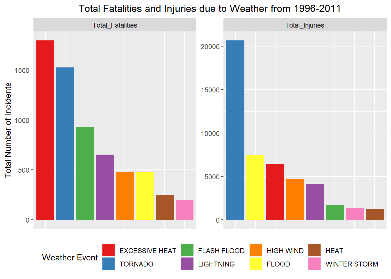
Plot Summary
These plots show the total amount of fatalities and injuries as a result of 8 weather events from 1996-2011. These weather events were chosen as they were in the 75th percentile of fatalities and injuries. Notice the scale between fatalities and injuries differs by abouta factor of 10 (Many more injuries than fatalities). Examination of the Fatalities plot shows that Excessive Heat, and Tornado are the largest contributors to fatalities, resulting in more than one thousand fatalities. In the total injuries plot, tornado, flood, and excessive heat produce that largest number of injuries.Based on this, Tornadoes seem to be the most harmful to population health as they result in large amounts of fatalities and massive amounts of injuries. Excessive heat is the next largest threat to health causing a large amount of fatalities and injuries. The hierarchy of weather events from here is less clear, but all the other weather events result in hundreds of fatalities and thousands of injuries.
Plots demonstrating harmful economic effects of Severe Weather events
costdata %>%
     gather(key,value,-EVTYPECOND) %>%
    ggplot(aes(x=reorder_within(EVTYPECOND,-value,key),y=value,
                           fill=EVTYPECOND))+
     geom_bar(stat="identity",position="dodge")+
    facet_wrap(~key,scales="free")+
    theme(axis.text.x=element_blank(),
          axis.ticks.x=element_blank(),
          axis.title.x = element_blank(),
          plot.title = element_text(hjust=.5),
          legend.position = "bottom")+
    scale_fill_brewer(palette = "Set2")+
    labs(y="Total Cost (in Dollars)",
         title = "Total Crop and Property Damage due to Weather from 1996-2011")+
    guides(fill=guide_legend(title="Weather Event"))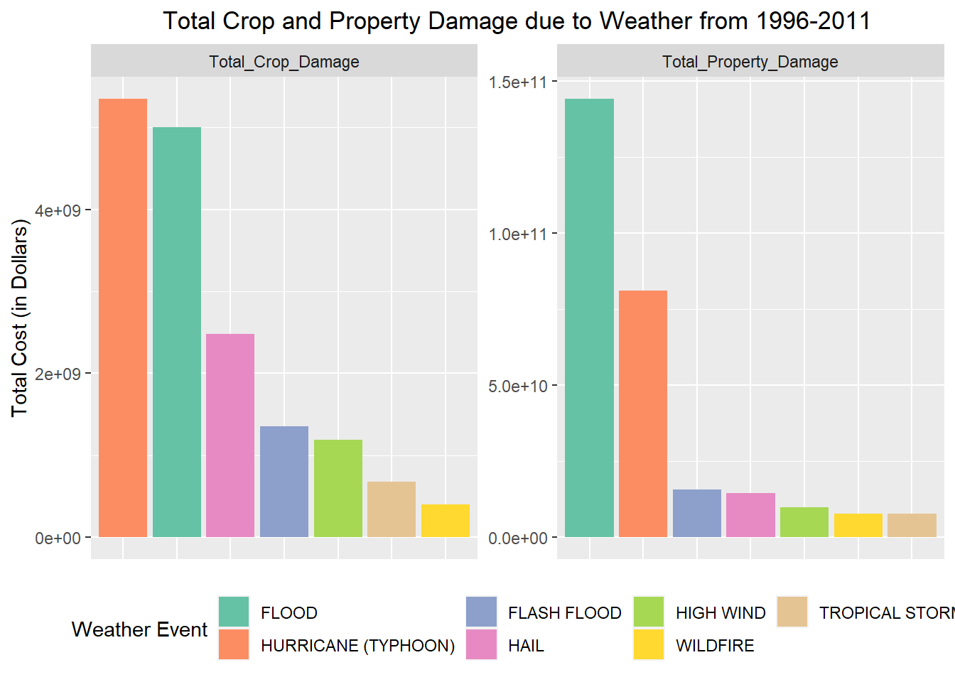
Plot Summary
This figure contains two plots, one showing the total crop damage and the other total property damage as a result of the most damaging weather events between 1996 and 2011. Notice that the scales of total crop damage and total property damage are very different, with total crop damage maxing out at slightly less than 6 billion dollars, whereas total property damage maxes out at slightly less than 150 billion dollars.
Total Crop Damage
In relation to total crop damage, hurricanes (typhoon) caused the largest amount of total crop damage resulting in approximately 5.5 billion dollars worth of damage. Floods were slightly less than this with about 5 billion dollars in damage. Hail was the next most crop damaging weather event causing about 2.5 billion dollars worth of damage. Flash floods and high winds were the next most damaging events causing a little over 1 billion dollars in crop damage. Finally tropical storms and wildfires were next resulting in hundreds of millions dollars worth of crop damage.
Total Property Damage
In relation to total property damage, Floods resulted in slightly less than 150 billion dollars worth of damage. The next most damaging weather event was hurricane (typhoon) coming in at around 80 billion dollars worth of property damage. Flash floods and hail were the next most damaging weather events resulting in approximately 15 billion dollars worth of damage. High winds caused almost 10 billion dollars worth of damage, while tropical storms and wildfires resulted in 7.5 billion dollars worth of damage.
Table of Economic and Population Health Consequences of Weather Events
For the interested reader who wants exact values for the variables of interest, I have also included this table which shows values for all weather events.
alltotal<-merge(totalstats,totalcost,by="EVTYPECOND",all=TRUE)
    datatable(alltotal,class="cell-border stripe")
This table shows the weather events that result in damage to population health or the economy between 1996 and 2011.