Weight Training Classification

Synopsis

The goal of this project is to correctly classify the quality of physical activity an individual carried out based on accelerometer collected from the belt, forearm, arm, and dumbbell. There were 5 different ways in which the exercise was carried out. It was done either exactly according to the specification (Class A), throwing the elbows to the front (Class B), lifting the dumbbell only halfway (Class C), lowering the dumbbell only halfway (Class D) and throwing the hips to the front (Class E). Class A is the correct manner in which the exercise should be carried out, while the other classes are common errors. Using the accelerometer data I was able to create a random forest model that classified this information into the 5 desired classes with 98 percent accuracy.

library(Hmisc)
library(vip)
library(randomForest)
library(e1071)
library(parallel)
library(MLmetrics)
library(foreach)
library(doParallel)
library(tidytext)
library(tidyverse)
library(reshape2)
library(caret)

Read in the Data

#train data location
fileurl<-"https://d396qusza40orc.cloudfront.net/predmachlearn/pml-training.csv"
if (!file.exists("fittrain.csv")){
    download.file(fileurl,"fittrain.csv",method="curl")
}
#test data location
fileurl<-"https://d396qusza40orc.cloudfront.net/predmachlearn/pml-testing.csv"
if (!file.exists("fittest.csv")){
    download.file(fileurl,"fittest.csv",method="curl")
}

# The data sets had many entries that were spaces ("") and thus I specified these
# to be missing values (NA)
fit_train<-read.csv("fittrain.csv",na.strings = c("NA",""))
fit_test<-read.csv("fittest.csv",na.strings = c("NA",""))

Assessing missing data

The first thing I want to do is assess the amount of missing data, so I know if there are certain predictors I should remove, or I should implement an imputation technique.

head(colSums(is.na(fit_train)),n=20)

##                    X            user_name raw_timestamp_part_1 
##                    0                    0                    0 
## raw_timestamp_part_2       cvtd_timestamp           new_window 
##                    0                    0                    0 
##           num_window            roll_belt           pitch_belt 
##                    0                    0                    0 
##             yaw_belt     total_accel_belt   kurtosis_roll_belt 
##                    0                    0                19216 
##  kurtosis_picth_belt    kurtosis_yaw_belt   skewness_roll_belt 
##                19216                19216                19216 
## skewness_roll_belt.1    skewness_yaw_belt        max_roll_belt 
##                19216                19216                19216 
##       max_picth_belt         max_yaw_belt 
##                19216                19216

Given a good number of these predictors are columns of missing values, I will go ahead and remove any predictor that is more than 95% missing values.

Removing Missing Values

threshold=.95
trainfilt<-fit_train[,colSums(is.na(fit_train))<(nrow(fit_train)*threshold)]
testfilt<-fit_test[,colSums(is.na(fit_test))<(nrow(fit_test)*threshold)]

Keeping accelerometer data

I am only using data from the accelerometers, as I am interested in assessing whether the acelerometers alone are enough to classify the quality with which an exercise is carried out. As a result, I will remove columns that contain other information.

trainfilt<-trainfilt[,-c(1,2,3,4,5,6,7)]
testfilt<-testfilt[,-c(1,2,3,4,5,6,7)]

trainfilt$classe<-as.factor(trainfilt$classe)
testfilt$classe<-as.factor(testfilt$classe)

Correlated Predictors

The next step in understanding the data is to look at correlations among the predictors. If variables are highly related to each other, it may be worthwhile to remove them or do some dimensionality reduction such as PCA. I use a correlation threshold of .75 here so as to only examine the most highly correlated predictors.

cormat<-trainfilt%>%
    select_if(is.numeric)%>%
    as.matrix()%>%
    rcorr(type='pearson')
highcor<-findCorrelation(cormat$r,cutoff = 0.75)
colnames(cormat$r[highcor,highcor])

##  [1] "accel_belt_z"      "roll_belt"         "accel_belt_y"     
##  [4] "accel_arm_y"       "total_accel_belt"  "accel_dumbbell_z" 
##  [7] "accel_belt_x"      "pitch_belt"        "magnet_dumbbell_x"
## [10] "accel_dumbbell_y"  "magnet_dumbbell_y" "accel_arm_x"      
## [13] "accel_dumbbell_x"  "accel_arm_z"       "magnet_arm_y"     
## [16] "magnet_belt_z"     "accel_forearm_y"   "gyros_forearm_y"  
## [19] "gyros_dumbbell_x"  "gyros_dumbbell_z"  "gyros_arm_x"

It is not surprising that there are many correlated predictors given that these are complex movements that require coordination from many parts of the body. Given this, it seems inappropriate to remove variables. Therefore I will go forward with a PCA technique in order to reduce the dimensionality of the data while still retaining the most informative aspects of the data.

Near Zero Variance

Next I will examine the data set to determine if there are any uninformative predictors and remove them if that is the case.

nzv<-nearZeroVar(trainfilt,saveMetrics = TRUE)
data.frame(zeroVar=sum(nzv$zeroVar==TRUE), NZV=sum(nzv$nzv==TRUE))

##   zeroVar NZV
## 1       0   0

There are no uninformative predictors, so the data is ready for modelling.

Validation data split

Before modelling, I split the training data set to include a validation set so the model does not overfit.

set.seed(1234)
samp<-createDataPartition(y=trainfilt$classe,p=.8,list = FALSE)
training<-trainfilt[samp,]
validation<-trainfilt[-samp,]

Model analysis

The model I am going to use is a random forest model since these typically have superior performance when it comes to classification. I am using a repeated cross validation procedure with 10 folds, and 3 repeats to get a stable model that minimizes overtraining. I will do a grid search to find the optimal value for the mtry parameter. This parameter corresponds to the number of variables randomly sampled as candidates at each split. I center and scale all the predictors and then do a pca selecting the components that account for 95% of the variance. I use a tree size of 250 as this is enough to produce stable accuracy and is not overly computationally intensive. Model performance will be assessed on its accuracy.

Data Preprocessing

control<-trainControl(method='repeatedcv',
                      number=10,
                      repeats = 3,
                      classProbs = TRUE,
                      summaryFunction = multiClassSummary,
                      allowParallel = TRUE,
                      savePredictions = TRUE,
                      search='grid',
                      verboseIter = TRUE)
tunevals<-expand.grid(.mtry=c(1:10))
#preprocess all datasets
trainpre<-preProcess(training,method=c('center','scale','pca'),thresh=.95)
trainpca<-predict(trainpre,training)
valpca<-predict(trainpre,validation)
testpca<-predict(trainpre,testfilt)

Random Forest Model Fit

#Parallelize the random forest process
cluster<-makeCluster(detectCores()-6) 
registerDoParallel(cluster)
set.seed(1234)
    rfmod<-train(classe~.,
                 data=trainpca,
                 method='rf',
                 ntree=250,
                 tuneGrid=tunevals,
                 verbose=TRUE,
                 metric='Accuracy',
                 trControl=control)

stopCluster(cluster)
registerDoSEQ()

Optimal mtry

This plot shows how the mtry value affects the cross validation accuracy for the model.

plot(rfmod)

This plot shows that an mtry value of 3 results in the highest accuracy on the held out cross validation sets.

Variable Importance

Using the vip plot we can assess what the most valuable predictors are.

vip(rfmod)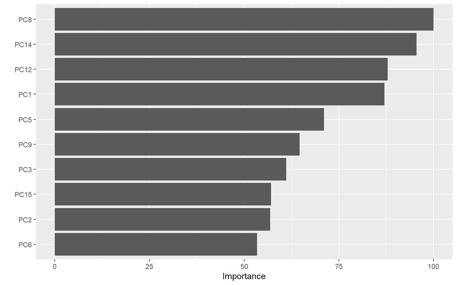

The most important predictor appears to be PC8, so let’s examine that to see what this component is capturing.

Principal Component Analysis

# Extract the pca loadings into an objects that will work with ggplot2
traincomp<-melt(trainpre$rotation)
colnames(traincomp)<-c("Original_Var","Component","Magnitude")

pcaplot<-traincomp %>%
  filter(Component %in% paste0("PC", c(8,14,12,1,5))) %>%
  ggplot(aes(Magnitude, Original_Var, fill = Original_Var)) +
  geom_col(show.legend = FALSE) +
  facet_wrap(~Component, nrow = 1) +
  labs(y = NULL,
       x="Strength of Contribution")
pcaplot

This figure shows the five most informative principal components and the contributions of each predictor into each principal component. Since each component is influenced in some way by each predictor, one way to understand what a component is capturing is by examining the tallest bars in the plot to see what predictors are contributing the most to each component. For example in PC 14 gyroscopic information from the belt in the z and y planes are the largest contributors. Given that one of the classes of exercises involved movement of the hips it makes sense this component would be useful for classification. The following plot shows the most informative predictors that contribute to these components to provide a clearer picture of what these components are capturing.

pcaplot2<-traincomp %>%
    filter(Component %in% paste0("PC", c(8,14,12,1,5))) %>%
    group_by(Component) %>%
    top_n(8, abs(Magnitude)) %>%
    ungroup() %>%
    mutate(Original_Var = reorder_within(Original_Var, abs(Magnitude), Component)) %>%
    ggplot(aes(abs(Magnitude), Original_Var, fill = Magnitude)) +
    geom_col() +
    scale_fill_viridis_c() +
    facet_wrap(~Component, scales = "free_y") +
    scale_y_reordered() +
    labs(
         title="Predictor Contribution  to  Top Five Principal Components",
        x = "Absolute value of contribution",
        y = NULL, fill = "Strength of \nContribution"
     ) +
    theme(plot.title=element_text(hjust=.5))
pcaplot2

The strongest predictors that were combined in the 5 most informative principal components are presented in the figure above. Green and yellow colors indicate positive values, while blue and purple colors indicate negative values. The strongest component, PC8, is capturing gyroscopic information from the dumbbell, and the overall acceleration in the forearm arm and forearm in z plane, vs. overall acceleration of the arm, in addition to the magnitude and acceleration of the forearm in the x plane. It makes sense that this is the most important component given it captures so much information about the dumbbell position and the forearm. Both of these are key factors in delineating between correctly and incorrectly carrying out the bicep curl.

ggplot(trainpca,aes(x=PC8,y=PC14,color=classe))+
  geom_point(alpha=.3)+
  scale_color_brewer(name="Exercise Type",
                        labels=c("Correct (A)","Elbows Front (B)","Half Curl Lift (C)",
                                 "Half Curl Lower (D)","Hips Front (E)"),
                     type="qual",palette = "Dark2")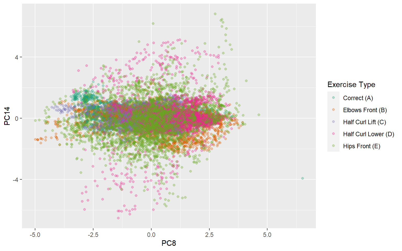

This plot is another way to demonstrate what the two most important principal components are capturing. Since there are so many components and many outcome categories, there are no explicit cutoffs where one component perfectly captures one exercise type. Instead there is a much more complex interaction among the components. PC14 does a relatively good job of capturing some component of exercises where the hips move forward, and the lowering of the dumbbell from halfway. Since PC14 is mainly dominated by gyroscopic information from the belt it makes sense that it would be better at classifying these two types of activities. In the next section I will examine the quality of the model fits.

Model Fit Evaluation

Confusion matrix-caret hold out cross validation data set

To assess the model fit I will be using confusion matrices. First I will examine the model fit to the held out re-samples in the caret cross validation procedure. Then I will examine the model performance against the validation set that I set aside before beginning the modelling.

confusionMatrix(rfmod)

## Cross-Validated (10 fold, repeated 3 times) Confusion Matrix 
## 
## (entries are percentual average cell counts across resamples)
##  
##           Reference
## Prediction    A    B    C    D    E
##          A 28.2  0.3  0.1  0.0  0.0
##          B  0.1 18.8  0.2  0.0  0.1
##          C  0.1  0.2 17.0  0.7  0.2
##          D  0.0  0.0  0.2 15.6  0.1
##          E  0.0  0.0  0.0  0.0 18.0
##                             
##  Accuracy (average) : 0.9767

On the cross validation set within the caret procedure, the model is quite accurate (~97%) with few observations off the diagonals.

Confusion matrix-validation data set

confusionMatrix(predict(rfmod,valpca),valpca$classe)

## Confusion Matrix and Statistics
## 
##           Reference
## Prediction    A    B    C    D    E
##          A 1111   10    1    1    0
##          B    1  744   12    0    0
##          C    2    4  657   25    7
##          D    2    0   12  617    6
##          E    0    1    2    0  708
## 
## Overall Statistics
##                                          
##                Accuracy : 0.9781         
##                  95% CI : (0.973, 0.9824)
##     No Information Rate : 0.2845         
##     P-Value [Acc > NIR] : < 2.2e-16      
##                                          
##                   Kappa : 0.9723         
##                                          
##  Mcnemar's Test P-Value : NA             
## 
## Statistics by Class:
## 
##                      Class: A Class: B Class: C Class: D Class: E
## Sensitivity            0.9955   0.9802   0.9605   0.9596   0.9820
## Specificity            0.9957   0.9959   0.9883   0.9939   0.9991
## Pos Pred Value         0.9893   0.9828   0.9453   0.9686   0.9958
## Neg Pred Value         0.9982   0.9953   0.9916   0.9921   0.9960
## Prevalence             0.2845   0.1935   0.1744   0.1639   0.1838
## Detection Rate         0.2832   0.1897   0.1675   0.1573   0.1805
## Detection Prevalence   0.2863   0.1930   0.1772   0.1624   0.1812
## Balanced Accuracy      0.9956   0.9881   0.9744   0.9767   0.9905

On the validation dataset the model performs fantastic. The model still achieves ~98% accuracy with few observations off the diagonal. The sensitivity of the model is quite high across all classes with .96 being the lowest. Specificity is .99 across all classes. Thus, the model is achieving high accuracy across all classes and is not suffering in its ability to classify one movement over another.

rfpred<-predict(rfmod,testpca)
# Calculate accuracy on the test set
sum(rfpred==testfilt$classe)/nrow(testfilt)*100

## [1] 100

Conclusion

With the validation set the model performs very well with an accuracy of ~98%. Thus the model has an out of sample error of 2 percent. Given the small size of the test set, the model performs with 100 percent accuracy. Thus this accelerometer data serves as an excellent source of information to classify the quality of an exercise.